9 The Snake Lemma without self-duality
9.1 The two hypotheses
A 2-z-exact 2-category satisfies condition \(\textup{(DPN)}\)—dinversion preserves normality—when for every antinormal pair \((m,e)\) the composite \(e\circ m\) is normal if and only if the dinversion \(w=2\text{-}\mathrm{coker}(m)\circ 2\text{-}\mathrm{ker}(e)\) is normal.
A 2-di-exact 2-category satisfies \(\textup{(DPN)}\); and a 2-z-exact 2-category satisfying \(\textup{(DPN)}\) is homologically self-dual.
Under (DI2) both sides of the biconditional hold outright: the composite \(e\circ m\) is antinormal by definition, and so is the dinversion \(w\), being the normal 2-monomorphism \(2\text{-}\mathrm{ker}(e)\) followed by the normal 2-epimorphism \(2\text{-}\mathrm{coker}(m)\); so both are normal, as observed in Proposition 6.3.
For the second assertion, let \((m,e)\) be an antinormal decomposition of the zero map. A null morphism is normal, by Proposition 4.13, so \(e\circ m\) is normal, and \(\textup{(DPN)}\) makes \(w\) normal. That is homological self-duality.
A 2-category satisfies condition \(\textup{(NEC)}\) when the composite of two normal 2-epimorphisms is a normal 2-epimorphism.
Both implications of Proposition 9.3 are strict. That the second is, Section 9.21 shows: \(\mathit{AbCat}\) is homologically self-dual and satisfies \(\textup{(NEC)}\) and its dual, and does not satisfy \(\textup{(DPN)}\) (Corollary 9.26); in dimension one the category \(\mathsf{CMon}\) of commutative monoids does the same [ 1 , Example 4.2.1 ] , and the 2-category \(\mathit{Sup}\) of complete lattices does the same with a five-element witness, the pentagon (Proposition 8.38). That the first is, dimension one already shows: for a field \(F\), the category of short exact sequences of \(F\)-vector spaces satisfies \(\textup{(DPN)}\) and is not di-exact [ 1 , Example 4.3.8 ] , so under the dictionary of Section 2.1 it is a 2-category that satisfies \(\textup{(DPN)}\) and not (DI2). Section 9.28 strengthens that witness to a 2-category which is not locally discrete: the 2-category of Hilbert lattices satisfies \(\textup{(DPN)}\) and not (DI2) (Theorem 9.32).
The two sets of hypotheses—(DI2) on the one side, \(\textup{(DPN)}\) together with \(\textup{(NEC)}\) on the other—are incomparable, and dimension one already shows it. The proof of [ 4 ] that Section 9.18 lifts is carried out in a homological category in the sense of that book: pointed, regular and protomodular. There the normal epimorphisms are the regular epimorphisms, so \(\textup{(NEC)}\) holds; the normal monomorphisms are not closed under composition, since normality of subgroups is not transitive—in the dihedral group \(D_{4}=\langle r,s\mid r^{4}=s^{2}=1,\; srs=r^{-1}\rangle \), the subgroup \(\langle s\rangle \) is normal in \(\langle s,r^{2}\rangle \), which is normal in \(D_{4}\), whereas \(\langle s\rangle \) is not. Di-exactness is exactly the further demand that turns that setting into the semi-abelian one: a homological category with binary coproducts is semi-abelian if and only if it is di-exact [ 19 , Theorem 5.7.3 with Definition 5.1.1 ] ; compare with the “old” axiom (SA*6) in the foundational article [ 12 ] .
The separation runs in both directions. On the one hand \(\mathsf{Grp}\) is semi-abelian, hence di-exact, and di-exactness is self-dual, so \(\mathsf{Grp}^{\operatorname {op}}\) is di-exact as well; but \(\textup{(NEC)}\) in \(\mathsf{Grp}^{\operatorname {op}}\) asks that normal monomorphisms of \(\mathsf{Grp}\) be closed under composition, which the subgroups above refute. On the other hand the category \(\mathsf{SES}(\mathsf{Vect}_{F})\) of short exact sequences of vector spaces over a field \(F\) satisfies \(\textup{(DPN)}\) and is not di-exact [ 1 , Example 4.3.8 ] , and it satisfies \(\textup{(NEC)}\): identify it with the category of pairs \((V,W)\) of a vector space and a subspace, in which kernels are computed componentwise while cokernels are computed componentwise in the category of morphisms of vector spaces and then reflected along the image factorisation. The normal epimorphisms out of \((V,W)\) are then exactly the morphisms
one for each subspace \(U\subseteq V\), being the cokernels of the normal monomorphisms \((U,U\cap W)\rightarrowtail (V,W)\); and the composite of the one for \(U\) with the one for \(U'/U\) is the one for \(U'\). Read as locally discrete 2-categories, \(\mathsf{Grp}^{\operatorname {op}}\) and \(\mathsf{SES}(\mathsf{Vect}_{F})\) therefore separate the hypotheses of this section from the hypothesis of Section 6, in both directions at once.
9.7 Why \(\textup{(DPN)}\) alone is not enough
Let \(A\xrightarrow []{a}B\xrightarrow []{b}C\) be a short 2-exact sequence in a 2-z-exact 2-category satisfying \(\textup{(DPN)}\), and let \(g\colon B\to Y\) be a morphism. Then \(b\circ 2\text{-}\mathrm{ker}(g)\) is normal if and only if \(2\text{-}\mathrm{coim}(g)\circ a\) is.
The pair \((2\text{-}\mathrm{ker}(g),b)\) is antinormal, \(2\text{-}\mathrm{ker}(g)\) being a normal 2-monomorphism and \(b\) a normal 2-epimorphism, and its composite is \(b\circ 2\text{-}\mathrm{ker}(g)\). Its dinversion is \(2\text{-}\mathrm{coker}(2\text{-}\mathrm{ker}(g))\circ 2\text{-}\mathrm{ker}(b)\), that is \(2\text{-}\mathrm{coim}(g)\circ a\), since \(a=2\text{-}\mathrm{ker}(b)\) and \(2\text{-}\mathrm{coim}(g)\) is by definition a 2-cokernel of \(2\text{-}\mathrm{ker}(g)\). Now apply Definition 9.2.
9.9 Two normal morphisms
The composite \(e\mathrel {:=}2\text{-}\mathrm{coim}(h)\circ b\colon B\to 2\text{-}\mathrm{Im}(h)\) is a normal 2-epimorphism; the composite \(e\circ 2\text{-}\mathrm{ker}(g)\) is null; and there is a normal 2-epimorphism \(t\colon 2\text{-}\mathrm{Im}(g)\to 2\text{-}\mathrm{Im}(h)\) with
The morphism \(b\) is a normal 2-epimorphism, being a 2-cokernel of \(a\), and \(2\text{-}\mathrm{coim}(h)\) is one because \(h\) is normal; so \(e\) is a normal 2-epimorphism by \(\textup{(NEC)}\). This is the only use of that hypothesis.
Next, \(h\circ b\circ 2\text{-}\mathrm{ker}(g)\cong d\circ g\circ 2\text{-}\mathrm{ker}(g)\cong 0\), by \(\psi \) and the structure 2-cell of \(2\text{-}\mathrm{ker}(g)\). Since \(h\cong 2\text{-}\mathrm{im}(h)\circ 2\text{-}\mathrm{coim}(h)\) and \(2\text{-}\mathrm{im}(h)\) reflects null morphisms, by Proposition 2.16, we get \(e\circ 2\text{-}\mathrm{ker}(g)\cong 0\). As \(2\text{-}\mathrm{coim}(g)\) is a 2-cokernel of \(2\text{-}\mathrm{ker}(g)\), this induces \(t\) with \(t\circ 2\text{-}\mathrm{coim}(g)\cong e\); and \(t\) is a normal 2-epimorphism by the dual of part (ii) of Proposition 3.6, the 2-epimorphism \(2\text{-}\mathrm{coim}(g)\) cancelling off the normal 2-epimorphism \(e\).
Finally
and \(2\text{-}\mathrm{coim}(g)\) is a 2-epimorphism, so \(2\text{-}\mathrm{im}(h)\circ t\cong d\circ 2\text{-}\mathrm{im}(g)\).
There is a morphism \(\kappa \colon 2\text{-}\mathrm{Ker}(t)\to X\), essentially unique with the property \(c\circ \kappa \cong 2\text{-}\mathrm{im}(g)\circ 2\text{-}\mathrm{ker}(t)\), and it is a 2-kernel of \(2\text{-}\mathrm{coker}(g)\circ c\). In particular \(\kappa \) is a normal 2-monomorphism.
By Lemma 9.10, \(d\circ 2\text{-}\mathrm{im}(g)\circ 2\text{-}\mathrm{ker}(t)\cong 2\text{-}\mathrm{im}(h)\circ t\circ 2\text{-}\mathrm{ker}(t)\cong 0\); as \(c=2\text{-}\mathrm{ker}(d)\), this produces \(\kappa \) with \(c\circ \kappa \cong 2\text{-}\mathrm{im}(g)\circ 2\text{-}\mathrm{ker}(t)\), essentially unique because \(c\) is a 2-monomorphism. The diagram
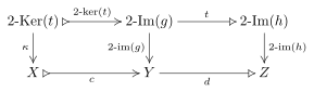
is then a morphism of short 2-exact sequences: its upper row is short 2-exact because \(t\) is a normal 2-epimorphism, hence a 2-cokernel of its 2-kernel by Proposition 3.11; its lower row is the lower row of 6.9; its left square commutes by the choice of \(\kappa \) and its right square by Lemma 9.10; and no coherence condition arises, by Proposition 3.26.
Its right vertical \(2\text{-}\mathrm{im}(h)\) is a 2-monomorphism, so Proposition 5.7 makes the left square a bipullback. The morphism \(\kappa \) is a 2-monomorphism, since \(c\circ \kappa \cong 2\text{-}\mathrm{im}(g)\circ 2\text{-}\mathrm{ker}(t)\) is a composite of two 2-monomorphisms and \(c\) is a 2-monomorphism, so that part (i) of Proposition 3.6 applies. Finally \(2\text{-}\mathrm{im}(g)\) is a normal 2-monomorphism, hence the 2-kernel of its own 2-cokernel, and that 2-cokernel is \(2\text{-}\mathrm{coker}(g)\) by Proposition 3.9, the morphism \(2\text{-}\mathrm{coim}(g)\) being a 2-epimorphism. So Proposition 5.4, applied to the left square with \(w=2\text{-}\mathrm{coker}(g)\), exhibits \(\kappa \) as a 2-kernel of \(2\text{-}\mathrm{coker}(g)\circ c\).
The composite \(2\text{-}\mathrm{coker}(g)\circ c\) is normal; its normal image factorisation may be written \(\mu \circ 2\text{-}\mathrm{coker}(\kappa )\) with \(\mu \colon 2\text{-}\mathrm{Cok}(\kappa )\to 2\text{-}\mathrm{Cok}(g)\) a normal 2-monomorphism. The morphism \(\underline{c}\) is normal.
The pair \((c,2\text{-}\mathrm{coker}(g))\) is antinormal: \(c\) is a normal 2-monomorphism, being a 2-kernel of \(d\), and \(2\text{-}\mathrm{coker}(g)\) is a normal 2-epimorphism. Its dinversion is \(2\text{-}\mathrm{coker}(c)\circ 2\text{-}\mathrm{ker}(2\text{-}\mathrm{coker}(g))\). Here \(2\text{-}\mathrm{coker}(c)\simeq d\), the lower row of 6.9 being short 2-exact, and \(2\text{-}\mathrm{ker}(2\text{-}\mathrm{coker}(g))\simeq 2\text{-}\mathrm{im}(g)\), as in the proof of Proposition 9.11. So the dinversion is \(d\circ 2\text{-}\mathrm{im}(g)\cong 2\text{-}\mathrm{im}(h)\circ t\), by Lemma 9.10: a normal 2-epimorphism followed by a normal 2-monomorphism, hence normal. Condition \(\textup{(DPN)}\) now makes \(2\text{-}\mathrm{coker}(g)\circ c\) normal.
By Proposition 9.11 its 2-kernel is \(\kappa \). In any normal image factorisation the 2-epimorphism part is a 2-cokernel of that 2-kernel—this is the first step of the proof of Proposition 3.22—so we may take it to be \(2\text{-}\mathrm{coker}(\kappa )\), and write \(\mu \) for the accompanying normal 2-monomorphism.
Finally, \(\underline{c}\) is characterised by \(\underline{c}\circ 2\text{-}\mathrm{coker}(f)\cong 2\text{-}\mathrm{coker}(g)\circ c\), and \(2\text{-}\mathrm{coker}(f)\) is a 2-epimorphism; so \(\underline{c}\) is normal by the dual of Proposition 3.23.
The morphism \(\overline{b}\) is normal.
We produce an antinormal decomposition of \(\overline{b}\) whose dinversion is visibly normal, and appeal to \(\textup{(DPN)}\).
Since \(e\circ a\cong 2\text{-}\mathrm{coim}(h)\circ b\circ a\cong 0\), the morphism \(a\) factors as \(a\cong 2\text{-}\mathrm{ker}(e)\circ \alpha \) for an essentially unique \(\alpha \colon A\to 2\text{-}\mathrm{Ker}(e)\), and \(\alpha \) is a normal 2-monomorphism by part (ii) of Proposition 3.6. Since \(e\circ 2\text{-}\mathrm{ker}(g)\cong 0\), by Lemma 9.10, the morphism \(2\text{-}\mathrm{ker}(g)\) factors likewise as \(2\text{-}\mathrm{ker}(g)\cong 2\text{-}\mathrm{ker}(e)\circ m_1\) with \(m_1\colon 2\text{-}\mathrm{Ker}(g)\to 2\text{-}\mathrm{Ker}(e)\) a normal 2-monomorphism.
The rows \(A\xrightarrow []{a}B\xrightarrow []{b}C\) and \(2\text{-}\mathrm{Ker}(e)\xrightarrow []{2\text{-}\mathrm{ker}(e)}B\xrightarrow []{e}2\text{-}\mathrm{Im}(h)\) are short 2-exact and share the middle object \(B\); with verticals \(\alpha \) and \(2\text{-}\mathrm{coim}(h)\) they form a morphism of short 2-exact sequences with identity middle component. By Lemma 4.27 its comparison \(2\text{-}\mathrm{Cok}(\alpha )\to 2\text{-}\mathrm{Ker}(2\text{-}\mathrm{coim}(h))\) is an equivalence, and \(2\text{-}\mathrm{Ker}(2\text{-}\mathrm{coim}(h))\simeq 2\text{-}\mathrm{Ker}(h)\) by Proposition 3.9. Write
for the composite of \(2\text{-}\mathrm{coker}(\alpha )\) with that equivalence. It is a 2-cokernel of \(\alpha \) followed by an equivalence, hence a normal 2-epimorphism with 2-kernel \(\alpha \); and the characterisation of the comparison in Lemma 4.27 reads \(2\text{-}\mathrm{ker}(h)\circ e_1\cong b\circ 2\text{-}\mathrm{ker}(e)\).
The rows \(2\text{-}\mathrm{Ker}(g)\xrightarrow []{2\text{-}\mathrm{ker}(g)}B\xrightarrow []{2\text{-}\mathrm{coim}(g)}2\text{-}\mathrm{Im}(g)\) and \(2\text{-}\mathrm{Ker}(e)\xrightarrow []{2\text{-}\mathrm{ker}(e)}B\xrightarrow []{e}2\text{-}\mathrm{Im}(h)\) are short 2-exact and share the middle object \(B\) as well; their verticals are \(m_1\) and \(t\), by Lemma 9.10. The same lemma supplies an equivalence \(2\text{-}\mathrm{Cok}(m_1)\simeq 2\text{-}\mathrm{Ker}(t)\); write
for the composite of \(2\text{-}\mathrm{coker}(m_1)\) with it, a 2-cokernel of \(m_1\), with \(2\text{-}\mathrm{ker}(t)\circ \rho \cong 2\text{-}\mathrm{coim}(g)\circ 2\text{-}\mathrm{ker}(e)\).
Now \(\overline{b}\cong e_1\circ m_1\). Indeed
and \(2\text{-}\mathrm{ker}(h)\) is a 2-monomorphism. So \((m_1,e_1)\) is an antinormal pair with composite \(\overline{b}\), and its dinversion is \(\rho \circ \alpha \), up to the equivalences just used and hence up to Corollary 3.8.
It remains to see that \(\rho \circ \alpha \) is normal, and for that we compose with \(\kappa \):
so that \(\kappa \circ \rho \circ \alpha \cong f\), the morphism \(c\) being a 2-monomorphism. Now \(f\) is normal and \(\kappa \) is a 2-monomorphism, so \(\rho \circ \alpha \) is normal by Proposition 3.23. By \(\textup{(DPN)}\), the composite \(\overline{b}\cong e_1\circ m_1\) is normal.
The two normality statements Proposition 9.12 and Proposition 9.13 are what Section 6 extracted from (DI2) at its two sites, and they are obtained here at very different prices. The first is immediate once \(t\) exists, because the dinversion of \((c,2\text{-}\mathrm{coker}(g))\) is \(2\text{-}\mathrm{im}(h)\circ t\); the second needs the morphism \(\kappa \) of Proposition 9.11, and hence the bipullback argument of Section 5. This is the only place in the paper where a bipullback is used for anything beyond Section 5 itself.
9.15 The connecting 1-cell
There is a normal 2-monomorphism \(\lambda \colon 2\text{-}\mathrm{Im}(f)\to 2\text{-}\mathrm{Ker}(t)\) with \(\lambda \circ 2\text{-}\mathrm{coim}(f)\cong \rho \circ \alpha \) and \(\kappa \circ \lambda \cong 2\text{-}\mathrm{im}(f)\).
From \(\kappa \circ \rho \circ \alpha \circ 2\text{-}\mathrm{ker}(f)\cong f\circ 2\text{-}\mathrm{ker}(f)\cong 0\) and the fact that the 2-monomorphism \(\kappa \) reflects null morphisms (Proposition 2.16) we get \(\rho \circ \alpha \circ 2\text{-}\mathrm{ker}(f)\cong 0\). As \(2\text{-}\mathrm{coim}(f)\) is a 2-cokernel of \(2\text{-}\mathrm{ker}(f)\), this induces \(\lambda \) with \(\lambda \circ 2\text{-}\mathrm{coim}(f)\cong \rho \circ \alpha \). Then
and \(2\text{-}\mathrm{coim}(f)\) is a 2-epimorphism, so \(\kappa \circ \lambda \cong 2\text{-}\mathrm{im}(f)\). Since \(2\text{-}\mathrm{im}(f)\) is a normal 2-monomorphism and \(\kappa \) is a 2-monomorphism, part (ii) of Proposition 3.6 makes \(\lambda \) a normal 2-monomorphism.
There are equivalences
The first is Lemma 4.10, applied to the antinormal pair \((m_1,e_1)\) of Proposition 9.13, whose composite is \(\overline{b}\) and whose dinversion is \(\rho \circ \alpha \). The second is Proposition 3.9: \(\rho \circ \alpha \cong \lambda \circ 2\text{-}\mathrm{coim}(f)\) with \(2\text{-}\mathrm{coim}(f)\) a 2-epimorphism. For the third, \(\mu \circ v\circ 2\text{-}\mathrm{coker}(f)\cong \mu \circ 2\text{-}\mathrm{coker}(\kappa )\cong 2\text{-}\mathrm{coker}(g)\circ c\cong \underline{c}\circ 2\text{-}\mathrm{coker}(f)\) by Proposition 9.12, and \(2\text{-}\mathrm{coker}(f)\) is a 2-epimorphism, so \(\underline{c}\cong \mu \circ v\); as \(\mu \) is a 2-monomorphism, Proposition 3.9 gives \(2\text{-}\mathrm{Ker}(\underline{c})\simeq 2\text{-}\mathrm{Ker}(v)\).
9.18 The theorem
Let \(\mathit{L}\) be a 2-z-exact 2-category with a strong bizero object which satisfies \(\textup{(DPN)}\) and \(\textup{(NEC)}\). Then the conclusion of Theorem 6.9 holds: for every diagram 6.9 with 2-exact rows whose two squares commute up to invertible 2-cells and whose verticals \(f\), \(g\) and \(h\) are normal, there is a 1-cell \(\partial \) making the sequence 6.9 2-exact; and if \(a=2\text{-}\mathrm{ker}(b)\) then \(\overline{a}=2\text{-}\mathrm{ker}(\overline{b})\), dually for \(\underline{d}\).
The same holds if \(\textup{(NEC)}\) is replaced by its dual, that normal 2-monomorphisms be closed under composition.
Consider first the special case in which \(a=2\text{-}\mathrm{ker}(b)\) and \(d=2\text{-}\mathrm{coker}(c)\), the standing hypothesis of Sections 9.9 and 9.15. By Proposition 9.3 the 2-category is homologically self-dual, so the whole of Section 4 is available, as it was in Section 6.
The morphism \(\overline{b}\) is normal by Proposition 9.13 and \(\underline{c}\) is normal by Proposition 9.12. Applying Proposition 6.14 to 8—with \(q'=2\text{-}\mathrm{coker}(\overline{b})\), with the equivalence \(z\) of Lemma 9.17 and with \(m=2\text{-}\mathrm{ker}(\underline{c})\)—gives 2-exactness at \(2\text{-}\mathrm{Cok}(f)\) and, \(\overline{b}\) being normal, at \(2\text{-}\mathrm{Ker}(h)\). By Proposition 6.17 we have \(\overline{a}=2\text{-}\mathrm{ker}(\overline{b})\), so the pair \((\overline{a},\overline{b})\) is 2-exact at \(2\text{-}\mathrm{Ker}(g)\); dually \(\underline{d}=2\text{-}\mathrm{coker}(\underline{c})\), and since \(\underline{c}\) is normal the pair \((\underline{c},\underline{d})\) is 2-exact at \(2\text{-}\mathrm{Cok}(g)\), by Proposition 4.4. The six 1-cells of 6.9 are normal: \(\overline{a}\) and \(\underline{d}\) are a 2-kernel and a 2-cokernel, \(\overline{b}\) and \(\underline{c}\) are normal as just recalled, and \(\partial \) is a normal 2-epimorphism followed by a normal 2-monomorphism by construction.
The general case reduces to this one exactly as in Section 6.19. That reduction uses Lemma 6.20, Proposition 3.9 and Proposition 6.21, and by Remark 6.22 none of them needs more than the Pure Snake Lemma, which Proposition 9.3 makes available here.
For the last assertion, note that \(\textup{(DPN)}\) is self-dual: passing to the opposite 2-category interchanges normal 2-monomorphisms with normal 2-epimorphisms and 2-kernels with 2-cokernels, so it carries an antinormal pair to an antinormal pair, its composite to the composite and its dinversion to the dinversion. A 2-category satisfying \(\textup{(DPN)}\) in which normal 2-monomorphisms are closed under composition therefore has an opposite satisfying \(\textup{(DPN)}\) and \(\textup{(NEC)}\), to which the theorem just proved applies; and the snake sequence of the opposite is the snake sequence of the original read backwards.
The two proofs are not related by exchanging a hypothesis. Section 6 builds \(\partial \) from a pure configuration whose middle object is \(C\), and for that it needs the 2-image \(i\) of \(b\circ 2\text{-}\mathrm{ker}(g)\) as a normal 2-monomorphism. Knowing that \(\overline{b}\) is normal does not supply it: \(b\circ 2\text{-}\mathrm{ker}(g)\cong 2\text{-}\mathrm{ker}(h)\circ \overline{b}\), so passing from one to the other composes two normal 2-monomorphisms, which is the hypothesis dual to \(\textup{(NEC)}\). This is why the construction above uses pure configurations with middle objects \(B\) and \(X\) instead, and why Proposition 9.11 has to be proved at all.
9.21 \(\mathit{AbCat}\) is homologically self-dual but does not satisfy \(\textup{(DPN)}\)
In \(\mathit{AbCat}\), normal 2-monomorphisms are closed under composition, and so are normal 2-epimorphisms.
By Corollary 8.6 and Corollary 3.8 it is enough to treat the inclusions of Serre subcategories and the projections onto Serre quotients. If \(K\) is a Serre subcategory of \(L\) and \(L\) one of \(\mathsf{A}\), then \(K\) is one of \(\mathsf{A}\), since \(L\) is closed in \(\mathsf{A}\) under subobjects, quotients and extensions. Dually, a Serre subcategory of \(\mathsf{A}/S\) is \(q(T)\) for a unique Serre subcategory \(T\) of \(\mathsf{A}\) containing \(S\), and \((\mathsf{A}/S)/q(T)\simeq \mathsf{A}/T\) by Gabriel’s correspondence [ 9 , Chapter III ] ; under that equivalence the composite of the two projections is the projection onto \(\mathsf{A}/T\).
The 2-category \(\mathit{AbCat}\) is homologically self-dual.
Let \((m,e)\) be an antinormal decomposition of the zero map; by Corollary 8.6 and Corollary 3.8 we may take \(m\) to be the inclusion of a Serre subcategory \(K\) of an abelian category \(\mathsf{A}\) and \(e\) the projection \(q\colon \mathsf{A}\to \mathsf{A}/S\). That \(e\circ m\) is essentially null says exactly that every object of \(K\) becomes zero in \(\mathsf{A}/S\), that is, \(K\subseteq S\).
The dinversion is \(S\rightarrowtail \mathsf{A}\twoheadrightarrow \mathsf{A}/K\), which is normal if and only if the \(K\)-saturation \(S^{K}\) is a Serre subcategory. By Proposition 8.9 we have \(S\subseteq S^{K}\subseteq S\vee K\), and \(S\vee K=S\) because \(K\subseteq S\); so \(S^{K}=S\), which is a Serre subcategory.
The counterexample of Proposition 8.12 cannot also refute \(\textup{(DPN)}\), and the reason points at what does. The cyclic quiver \(1\to 2\to 1\) admits the rotation exchanging its two vertices, and \(\operatorname {rad}^{3}=0\) is preserved by it, so \(\Lambda \) has an automorphism carrying \(S_{1}\) to \(S_{2}\) and hence \(K\) to \(S\). The two saturations \(K^{S}\) and \(S^{K}\) are therefore carried into one another, and both fail to be Serre subcategories; the biconditional of Definition 9.2 holds vacuously at that pair. What is wanted is an algebra on the same quiver whose relations break the rotation.
The 2-category \(\mathit{AbCat}\) does not satisfy \(\textup{(DPN)}\).
Let \(\Bbbk \) be a field and let \(\mathsf{A}\) be the category of representations

of finite-dimensional \(\Bbbk \)-vector spaces subject to the single relation \(a\circ b=0\); no condition is imposed on \(b\circ a\). This is the category of finite-dimensional modules over \(\Lambda \mathrel {:=}\Bbbk Q/(\alpha \beta )\), where \(Q\) is the cyclic quiver \(1\xrightarrow {\alpha }2\xrightarrow {\beta }1\) and \(\alpha \beta \) is the path of length 2 from 2 to 2; so \(\mathsf{A}\) is abelian, with kernels and cokernels formed componentwise. The algebra \(\Lambda \) is five-dimensional, a quotient of the six-dimensional Nakayama algebra of Proposition 8.12: the relation forces every path of length 3 to vanish, and it is exactly the rotation symmetry of Remark 9.24 that it destroys. Put
the objects all of whose composition factors are \(\cong S_{1}\), respectively \(\cong S_{2}\); both are Serre subcategories, and \(K\vee S=\mathsf{A}\) since every object has finite length.
The \(K\)-saturation of \(S\) is a Serre subcategory. Let \(V\) be any object. Then \(N\mathrel {:=}(\ker a,0)\) is a subobject of \(V\), because \(a(\ker a)=0\) and \(b(0)\subseteq \ker a\), and it lies in \(K\). In the quotient \(V/N\) the map induced by \(a\) is injective and the relation still holds, so \(a\circ b=0\) forces \(b=0\) on \(V/N\); hence \((0,V_{2})\) is a subobject of \(V/N\) lying in \(S\), and the remaining quotient has zero first component, so lies in \(K\). This is a filtration of \(V\) with successive subquotients in \(K\), \(S\) and \(K\), so \(S^{K}=\mathsf{A}=K\vee S\), and Proposition 8.9 applies. Note that no finiteness was used.
The \(S\)-saturation of \(K\) is not. Let \(M\) be the representation with \(M_{1}=\langle x,z\rangle \), \(M_{2}=\langle y\rangle \), \(a(x)=y\), \(a(z)=0\) and \(b(y)=z\); the relation holds, since \(a(b(y))=a(z)=0\), whereas \(b(a(x))=z\neq 0\). A subobject \((W_{1},W_{2})\) with \(y\in W_{2}\) contains \(z=b(y)\), and if it contains \(x\) as well it is all of \(M\); a subobject with \(W_{2}=0\) has \(W_{1}\subseteq \ker a=\langle z\rangle \). So \(M\) is uniserial of length 3,
with successive subquotients \(S_{1}\), \(S_{2}\), \(S_{1}\); it is the indecomposable projective \(\Lambda e_{1}\). Let \(X_{1}\subseteq X_{2}\subseteq M\) be a filtration with \(X_{1}\in S\), \(X_{2}/X_{1}\in K\) and \(M/X_{2}\in S\). The three proper subobjects listed have first components \(0\), \(\langle z\rangle \) and \(\langle z\rangle \), of which only the first is zero, so \(X_{1}=0\); then \(X_{2}\in K\) leaves \(X_{2}=0\) or \(X_{2}=(\langle z\rangle ,0)\), and in either case \(M/X_{2}\) has nonzero first component and so does not lie in \(S\). By Definition 8.8 and Proposition 8.9, \(M\notin K^{S}\) and \(K^{S}\) is not a Serre subcategory.
Taking \(m\) to be the inclusion of \(K\) and \(e\) the projection onto \(\mathsf{A}/S\), the pair \((m,e)\) is antinormal, its dinversion \(S\rightarrowtail \mathsf{A}\twoheadrightarrow \mathsf{A}/K\) is normal and the composite \(e\circ m\) is not.
It is worth being explicit about which hypothesis gives way, since Proposition 9.22 disposes of the other one and of its dual. What fails in \(\mathit{AbCat}\) is the hypothesis that carries the mathematics, not the bookkeeping one; and by Proposition 9.8 it fails at both sites at once. The models of Section 8 are therefore not a luxury: they are the only two-dimensional 2-categories we know in which Theorem 6.9 applies; Section 9.28 adds a two-dimensional 2-category in which the Snake Lemma holds, but only in the form of Theorem 9.19.
9.28 A two-dimensional model: Hilbert lattices
Let \(\mathcal{C}\) be a class of complete lattices, closed under isomorphism, containing a one-element lattice, and such that every interval of a member of \(\mathcal{C}\) belongs to \(\mathcal{C}\). The full sub-2-category \(\mathit{Sup}_{\mathcal{C}}\) of \(\mathit{Sup}\) on \(\mathcal{C}\) is then 2-z-exact with a strong bizero object; Corollary 8.34 and Proposition 8.35 describe its normal 2-monomorphisms, its normal 2-epimorphisms and its antinormal morphisms, and both closure properties of Corollary 8.34 hold in it. Moreover, \(\mathit{Sup}_{\mathcal{C}}\) satisfies condition (DI2) if and only if every member of \(\mathcal{C}\) is modular, and condition \(\textup{(DPN)}\) if and only if every member of \(\mathcal{C}\) is transposition-symmetric.
The first assertions are proved exactly as Theorem 8.37. Down-segments, up-segments and intervals of a member of \(\mathcal{C}\) are intervals, so lie in \(\mathcal{C}\) up to isomorphism; hence the 2-kernels and 2-cokernels of Proposition 8.33, computed in \(\mathit{Sup}\), have their vertices in \(\mathit{Sup}_{\mathcal{C}}\), and since the sub-2-category is full, they are 2-kernels and 2-cokernels there. A one-element lattice is a strong bizero object as in Proposition 8.32, and Corollary 8.34 and Proposition 8.35 transfer, as they did for \(\mathit{Sup}_{\mathrm{mod}}\).
For (DI2): if every member of \(\mathcal{C}\) is modular, the argument of Theorem 8.37 applies verbatim; if some member \(L\) is not modular, the proof of Proposition 8.36 produces elements \(w\), \(v\) of \(L\) for which \(c_{w,v}\) is antinormal in \(\mathit{Sup}_{\mathcal{C}}\)—its two constituents have their vertices \({\downarrow }w\) and \({\uparrow }v\) in \(\mathcal{C}\)—and not normal.
For \(\textup{(DPN)}\): up to isomorphisms, which change nothing by Corollary 3.8, an antinormal pair of \(\mathit{Sup}_{\mathcal{C}}\) is of the form \(({\downarrow }a\to L,q_{b})\) for elements \(a\), \(b\) of a member \(L\), with composite \(c_{a,b}\), and as in the proof of Proposition 8.38 its dinversion is \(c_{b,a}\). By Proposition 8.35, whose factorisation passes through the interval \([a\wedge b,a]\) of \(L\), which lies in \(\mathcal{C}\), the composite is normal precisely when the transposition at \((a,b)\) is invertible, and the dinversion is normal precisely when the transposition at \((b,a)\) is. The biconditional of Definition 9.2 is therefore exactly transposition-symmetry of the members of \(\mathcal{C}\).
For elements \(a\), \(b\) of a complete lattice, the transposition \([a\wedge b,a]\to [b,a\vee b]\) is invertible if and only if \(\mathrm{M}(b,a)\) and \(\mathrm{M}^{*}(a,b)\) both hold. In particular, a complete lattice in which both the relation \(\mathrm{M}\) and the relation \(\mathrm{M}^{*}\) are symmetric is transposition-symmetric.
For \(x\in [a\wedge b,a]\) and \(z\in [b,a\vee b]\) we have \(x\vee b\leq z\) if and only if \(x\leq z\wedge a\), so the transposition and the monotone map \(z\mapsto z\wedge a\) in the opposite direction form an adjunction. The transposition is invertible if and only if the two composites are identities: in one direction because an invertible monotone map is left adjoint to its inverse and adjoints are unique, in the other because mutually inverse monotone bijections between complete lattices are isomorphisms of \(\mathit{Sup}\).
The first composite is the identity when \((x\vee b)\wedge a=x\) for all \(x\in [a\wedge b,a]\), which is \(\mathrm{M}(b,a)\): for \(c\leq a\) the element \(x=c\vee (a\wedge b)\) lies in \([a\wedge b,a]\) and satisfies \(x\vee b=c\vee b\), so the former condition yields \((c\vee b)\wedge a=c\vee (a\wedge b)\), and conversely. The second composite is the identity when \((z\wedge a)\vee b=z\) for all \(z\in [b,a\vee b]\), which is \(\mathrm{M}^{*}(a,b)\) by the dual translation. The final assertion holds since \(\mathrm{M}(b,a)\wedge \mathrm{M}^{*}(a,b)\) and \(\mathrm{M}(a,b)\wedge \mathrm{M}^{*}(b,a)\) are then each equivalent to \(\mathrm{M}(a,b)\wedge \mathrm{M}^{*}(a,b)\).
For closed subspaces \(A\), \(B\) of a Hilbert space \(H\), the transposition \([A\wedge B,A]\to [B,A\vee B]\) of \(\mathrm{L}(H)\) is invertible if and only if both \(A+B\) and \(A^{\perp }+B^{\perp }\) are closed. In particular, every Hilbert lattice is transposition-symmetric.
By Lemma 9.30, invertibility is the conjunction of \(\mathrm{M}(B,A)\) and \(\mathrm{M}^{*}(A,B)\). A theorem of Mackey identifies the dual modular pairs of \(\mathrm{L}(H)\): the condition \(\mathrm{M}^{*}(A,B)\) holds if and only if the vector sum \(A+B\) is closed [ 16 , Theorem III-6 ] ; see also [ 20 ] . The direction we shall use at Theorem 9.32 is elementary: if \(A+B\) is closed then \(A\vee B=A+B\), and for a closed \(C\supseteq B\), any \(x\in C\cap (A+B)\) is \(p+q\) with \(p\in A\) and \(q\in B\subseteq C\), so that \(p=x-q\in C\cap A\) and \(x\in (C\cap A)+B\subseteq (C\wedge A)\vee B\); the reverse inclusion holds in every lattice, and \(\mathrm{M}^{*}(A,B)\) follows. The converse is elementary as well, and is Mackey’s own argument: if \(A+B\) is not closed, choose \(x\in (A\vee B)\setminus (A+B)\) and test \(\mathrm{M}^{*}(A,B)\) at \(C=B+\langle x\rangle \), which is closed because a closed subspace and a line span a closed subspace; a nonzero multiple of \(x\) in \(C\cap A\) would return \(x\) to \(A+B\), so \(C\cap A\subseteq B\) and \((C\wedge A)\vee B=B\neq C\).
Orthocomplementation is an anti-automorphism of \(\mathrm{L}(H)\), turning joins into meets and reversing the order, so it carries the condition \(\mathrm{M}(B,A)\) to \(\mathrm{M}^{*}(B^{\perp },A^{\perp })\) [ 20 , Theorem 5(i) ] , which by Mackey’s theorem holds if and only if \(B^{\perp }+A^{\perp }\) is closed. The stated criterion follows, and it is symmetric in \(A\) and \(B\) because vector sums are. By a classical duality the two conditions are in fact equivalent to one another [ 14 , Theorem IV.4.8 ] , so that invertibility amounts to closedness of \(A+B\) alone; but the symmetry of the two-condition form is all we use.
The 2-category \(\mathit{Sup}_{\mathrm{hil}}\) of Hilbert lattices is 2-z-exact with a strong bizero object, its normal 2-monomorphisms and its normal 2-epimorphisms are closed under composition, and it satisfies condition \(\textup{(DPN)}\); but it is not 2-di-exact. The Snake Lemma holds in \(\mathit{Sup}_{\mathrm{hil}}\) in the form of Theorem 9.19, while Theorem 6.9 does not apply to it.
Everything except the failure of (DI2) is Proposition 9.29 combined with Proposition 9.31. For the failure, let \(H\) be infinite-dimensional, take an orthonormal sequence \((e_{n})_{n\geq 1}\), and consider the closed subspaces
The vectors \(b_{n}\) are pairwise orthogonal, so \(B\) consists of the sums \(\sum _{n}c_{n}b_{n}\) with square-summable coefficients, and \(A\wedge B=0\), since a vector of \(B\) lying in \(A\) has all coefficients \(\tfrac {c_{n}}{n}\) of the \(e_{2n-1}\) zero. The subspace \(A+B\) contains every \(e_{2n}\) and every \(e_{2n-1}=n(b_{n}-e_{2n})\), so \(v\mathrel {:=}\sum _{n}\tfrac {1}{n}\, e_{2n-1}\) lies in \(A\vee B\); but \(v\notin A+B\), since \(v=a+\sum _{n}c_{n}b_{n}\) forces \(c_{n}=1\) for every \(n\), which is not square-summable. Now \(Z\mathrel {:=}B\vee \langle v\rangle =B+\langle v\rangle \) is closed, being the sum of a closed subspace and a line, and \(Z\wedge A=0\): if \(\sum _{n}c_{n}b_{n}+tv\in A\), then comparing coefficients of \(e_{2n-1}\) gives \(c_{n}=-t\) for every \(n\), so \(t=0\), and the vector lies in \(B\wedge A=0\). Hence \((Z\wedge A)\vee B=B\), whereas \(Z\wedge (A\vee B)=Z\), which contains \(v\notin B\): the subspace \(Z\) witnesses the failure of \(\mathrm{M}^{*}(A,B)\). So the transposition at \((A,B)\) is not invertible by Lemma 9.30, the antinormal morphism \(c_{A,B}\) of \(\mathit{Sup}_{\mathrm{hil}}\) is not normal by Proposition 8.35, and (DI2) fails; by Proposition 8.36, \(\mathrm{L}(H)\) is not modular either. Finally, Theorem 9.19 applies by Proposition 9.3 and the above, whereas the hypothesis of Theorem 6.9 fails in \(\mathit{Sup}_{\mathrm{hil}}\).
Remark 9.5 separated \(\textup{(DPN)}\) from (DI2) by a locally discrete 2-category; Theorem 9.32 separates them by a 2-category whose 2-cells, the inequalities, carry the universal properties. The trade the two conditions embody is here concrete: condition (DI2) would ask every sum of closed subspaces to be closed, which is false, while \(\textup{(DPN)}\) asks only that the two sums attached to an antinormal pair and to its dinversion be closed together, which is Mackey’s symmetry. Once more the failure of (DI2) is a categorical construction creating something new—here the closure of a sum, in \(\mathit{AbCat}\) the extensions which a localisation creates (Remark 8.13).
In \(\mathit{Sup}_{\mathrm{hil}}\), Remark 8.40 reads almost word for word: the input of the Snake Lemma reduces to a normal 1-cell \(g\) together with closed subspaces \(U\), \(V\) such that \(g(U)\leq V\), the six terms of the snake sequence are again Hilbert lattices, and \(\partial \) may be taken to be \(g\) itself, restricted. The one difference is that the normality of the two outer verticals, which modularity provided for free, is now a genuine hypothesis—by Proposition 9.31 a pair of closed-sum conditions—and Remark 8.43 shows that it cannot be dropped.
The introduction of [ 11 ] observes that the homological categories of Banach and of Hilbert spaces are not modular—their lattices of normal subobjects are lattices of closed subspaces, “just orthomodular” [ 11 , 2.3.2 ] —so that their connected sequences of homology functors fail to be exact, and remarks that a deeper study of such settings could be of interest [ 11 , 0.4 ] . Theorem 9.32 may be read as a step in that study, taken from the two-dimensional side: what a Snake Lemma asks of \(\mathrm{L}(H)\) is not the modular law but Mackey’s symmetry, at the price of the non-self-dual pair of hypotheses. The projection lattices of von Neumann algebras stratify along the same line: for a finite factor the projection lattice is a continuous geometry [ 24 ] , hence modular and within \(\mathit{Sup}_{\mathrm{mod}}\), while \(\mathrm{L}(H)\) is the projection lattice of the type \(\mathrm{I}\) factor \(\mathcal{B}(H)\); whether the projection lattice of an arbitrary von Neumann algebra is transposition-symmetric we do not know.
A lattice of finite length which is transposition-symmetric is modular. Hence if every member of a class \(\mathcal{C}\) as in Proposition 9.29 is of finite length, then \(\mathit{Sup}_{\mathcal{C}}\) satisfies \(\textup{(DPN)}\) if and only if it satisfies (DI2).
Transposition-symmetry is inherited by intervals, the transpositions of a pair computed in an interval agreeing with those computed in the ambient lattice, and it is invariant under dualisation: the transposition of \(L^{\operatorname {op}}\) at \((a,b)\) is the right adjoint \(z\mapsto z\wedge b\colon [a,a\vee b]\to [a\wedge b,b]\) of the transposition of \(L\) at \((b,a)\), and an adjoint is invertible precisely when its partner is. Call \(L\) semimodular when \(a\succ a\wedge b\) implies \(a\vee b\succ b\) for all \(a\), \(b\), where \(x\succ y\) means that \(x\) covers \(y\); a lattice of finite length which is semimodular and dually semimodular is modular [ 2 , Chapter II, Theorem 16 ] . By the invariance under dualisation it therefore suffices to prove that \(L\) is semimodular.
Let \(a\succ a\wedge b\) and suppose, for a contradiction, that \(a\vee b\not\succ b\). We work in the interval \([a\wedge b,a\vee b]\) and write \(\bot \) and \(\top \) for its bounds; thus \(a\) is an atom there, \(a\wedge b=\bot \) and \(a\vee b=\top \), while \(\top \not\succ b\). The transposition at \((a,b)\) goes from the two-element chain \([\bot ,a]\) to the interval \([b,\top ]\), which has at least three elements, so it is not invertible; its unit is nevertheless trivial, since \((\bot \vee b)\wedge a=\bot \) and \((a\vee b)\wedge a=a\), so by the proof of Lemma 9.30 its counit fails: there is \(w\in [b,\top ]\) with \((w\wedge a)\vee b{\lt}w\). Were \(w\wedge a=a\), then \(w\geq a\vee b=\top \) and the counit would hold at \(w\); so \(w\wedge a=\bot \), and \(b{\lt}w{\lt}\top \). Every \(t\) with \(w\leq t{\lt}\top \) satisfies \(t\wedge a=\bot \)—otherwise \(a\leq t\), whence \(t\geq a\vee w\geq a\vee b=\top \)—as well as \(t\vee a=\top \); since the length is finite, we may ascend from \(w\) to a coatom \(B\), with \(b{\lt}B\), \(B\wedge a=\bot \) and \(B\vee a=\top \). The transposition at \((B,a)\), from \([\bot ,B]\) to \([a,\top ]\), is not invertible, its unit failing at \(b\): \((b\vee a)\wedge B=\top \wedge B=B\neq b\). By transposition-symmetry, the transposition at \((a,B)\) is not invertible either. But it is the map \(\{ \bot ,a\} \to \{ B,\top \} \) sending \(\bot \) to \(B\) and \(a\) to \(\top \), an isomorphism of two-element chains—a contradiction.
The separation of \(\textup{(DPN)}\) from (DI2) within \(\mathit{Sup}\) is thus an intrinsically infinite phenomenon: no lattice of finite length, indeed no class of them, can witness it. The proof of Proposition 9.34 locates the tension. An atom \(a\) and a coatom \(B\) with \(a\not\leq B\) always transpose invertibly from \(a\) to \(B\), so transposition-symmetry forces \([\bot ,B]\cong [a,\top ]\), a strong homogeneity which a finite non-modular lattice cannot sustain. The Hilbert lattices can, because the sum of a closed subspace with a finite-dimensional one is always closed: closedness of sums, and with it invertibility of transpositions, only fails in infinite dimensions, out of reach of the covering argument.